Stimulus optimization

This script shows how to optimize the stimulus presentation by means of selecting the optimal subset of stimuli from a set of candidate stimuli and how to select an optimal layout to allocate them to a stimulus grid. For more information on the optimization of such subset and layout, see [1].

References

[1]

Thielen, J., Van Den Broek, P., Farquhar, J., & Desain, P. (2015). Broad-Band visually evoked potentials: re(con)volution in brain-computer interfacing. PloS one, 10(7), e0133797. DOI: https://doi.org/10.1371/journal.pone.0133797

import matplotlib.pyplot as plt
import numpy as np

import pyntbci

Simulate data

The cell below simulates some synthetic c-VEP data in response to a circularly shifted m-sequence.

FS = 120
PR = 60
SHIFT = 2

v = pyntbci.stimulus.make_m_sequence()
SHIFTS = np.arange(0, v.shape[1], SHIFT)
V = pyntbci.stimulus.shift(v, SHIFT)
V = np.repeat(V, FS // PR, axis=1)
N_CLASSES = V.shape[0]
CYCLE_SIZE = V.shape[1] / FS
LAGS = SHIFTS / PR

N_TRIALS = 1 * N_CLASSES
N_CHANNELS = 16
N_SAMPLES = int(2 * CYCLE_SIZE * FS)
N_COMPONENTS = 3
N_FILTER_BANDS = 4
ENCODING_LENGTH = 0.3
SEED = 42

X, y, V = pyntbci.eeg.generate_c_vep(
    N_TRIALS, N_CHANNELS, N_SAMPLES, FS, n_classes=N_CLASSES, stimulus=V, primary_channels=8, random_state=SEED
)

Extract templates with rCCA

rcca = pyntbci.classifiers.rCCA(stimulus=V, fs=FS, event="id", encoding_length=0.3)
rcca.fit(X, y)
T = rcca.Ts_[:, 0, :].T

Optimize stimulus subset

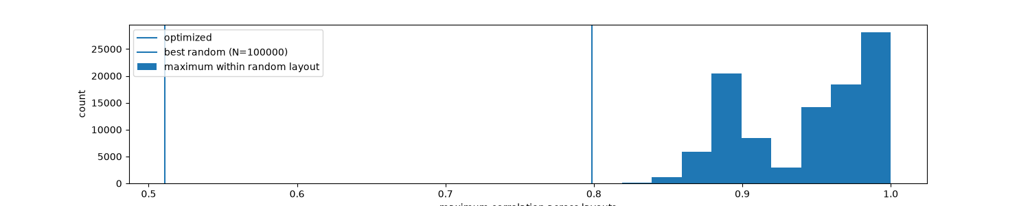
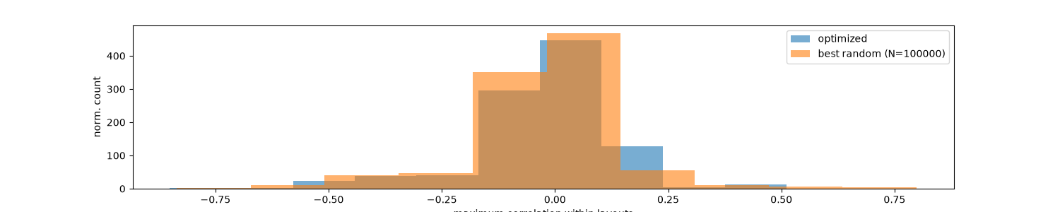
The cell above generated 63 different codes and for each an expected template EEG response. In the following we assume we have a 4 x 8 matrix speller setup, for a total of 32 classes. Thus, we can select an optimal subset of 32 codes from the 63 available codes. This we will do by minimizing the maximum pair-wise correlation between templates within the subset.

n_random = 100000  # number of random "optimizations"

# Assumed speller matrix
matrix = np.arange(N_CLASSES).reshape(4, 8)
n_classes = matrix.size

# Compute correlation matrix
rho = pyntbci.utilities.correlation(T, T)
rho[np.eye(rho.shape[0]) == 1] = np.nan

# Optimize subset
optimized_subset = pyntbci.stimulus.optimize_subset_clustering(T, n_classes)
optimized = np.nanmax(rho[optimized_subset, :][:, optimized_subset])
optimized_vals = rho[optimized_subset, :][:, optimized_subset].flatten()
optimized_vals = optimized_vals[~np.isnan(optimized_vals)]

# Random subset
random_subset = []
value = 1  # maximum correlation
random = np.zeros(n_random)
for i in range(n_random):
    subset_ = np.random.permutation(T.shape[0])[:n_classes]
    random[i] = np.nanmax(rho[subset_, :][:, subset_])
    if random[i] < value:
        random_subset = subset_
        value = random[i]
random_vals = rho[random_subset, :][:, random_subset].flatten()
random_vals = random_vals[~np.isnan(random_vals)]

# Visualize tested and optimized layouts
plt.figure(figsize=(15, 3))
plt.axvline(optimized, label="optimized")
plt.axvline(random.min(), label=f"best random (N={n_random})")
plt.hist(random, label="maximum within random layout")
plt.legend()
plt.xlabel("maximum correlation across layouts")
plt.ylabel("count")

# Visualize optimized layouts
plt.figure(figsize=(15, 3))
plt.hist(optimized_vals, 10, alpha=0.6, label="optimized")
plt.hist(random_vals, 10, alpha=0.6, label=f"best random (N={n_random})")
plt.legend()
plt.xlabel("maximum correlation within layouts")
plt.ylabel("norm. count")

• 
• 

Text(145.22222222222223, 0.5, 'norm. count')

Optimize stimulus layout

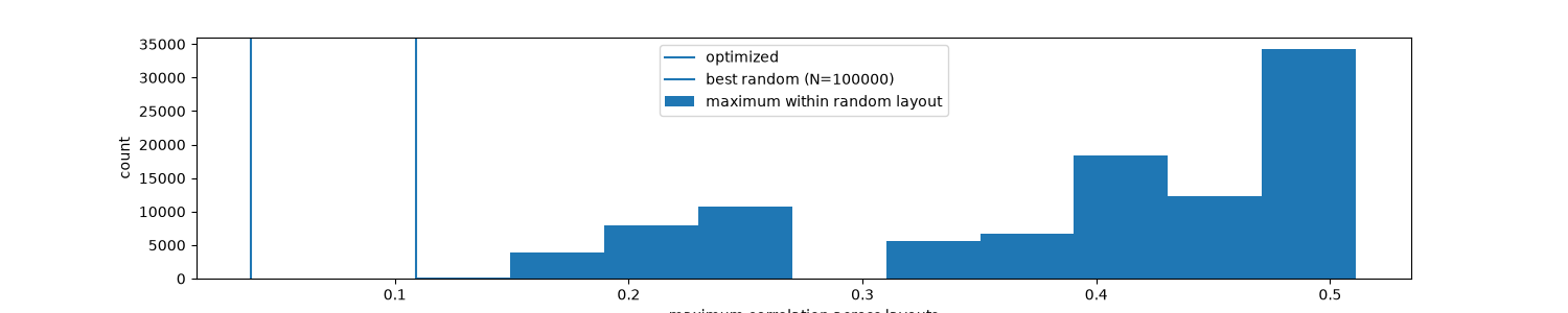
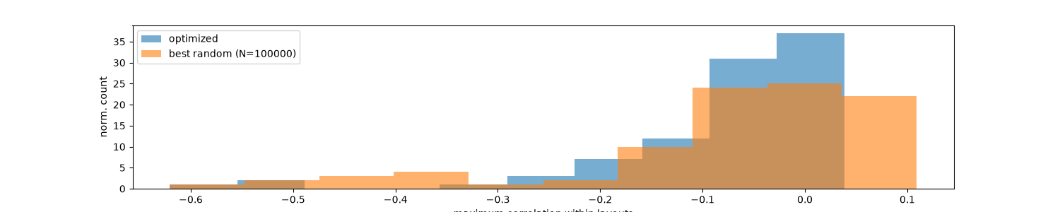
Now we have the optimal subset of 32 codes. Still, we could optimize how these are allocated to the 4 x 8 speller grid, such that codes that still correlate much are not placed at neighbouring cells in the grid.

# Select optimize subset
T = T[optimized_subset, :]

# Compute correlation matrix
rho = pyntbci.utilities.correlation(T, T)
rho[np.eye(rho.shape[0]) == 1] = np.nan

# Create neighbours matrix assuming 4 x 8 grid
neighbours = pyntbci.utilities.find_neighbours(matrix)

# Optimize layout
optimized_layout = pyntbci.stimulus.optimize_layout_incremental(T, neighbours, 50, 50)
optimized = np.nanmax(rho[optimized_layout[neighbours[:, 0]], optimized_layout[neighbours[:, 1]]])
optimized_vals = rho[optimized_layout[neighbours[:, 0]], optimized_layout[neighbours[:, 1]]].flatten()
optimized_vals = optimized_vals[~np.isnan(optimized_vals)]

# Random layout
random_layout = []
value = 1  # maximum correlation
random = np.zeros(n_random)
for i in range(n_random):
    layout_ = np.random.permutation(T.shape[0])
    random[i] = np.nanmax(rho[layout_[neighbours[:, 0]], layout_[neighbours[:, 1]]])
    if random[i] < value:
        random_layout = layout_
        value = random[i]
random_vals = rho[random_layout[neighbours[:, 0]], random_layout[neighbours[:, 1]]].flatten()
random_vals = random_vals[~np.isnan(random_vals)]

# Visualize tested and optimized layouts
plt.figure(figsize=(15, 3))
plt.axvline(optimized, label="optimized")
plt.axvline(random.min(), label=f"best random (N={n_random})")
plt.hist(random, label="maximum within random layout")
plt.legend()
plt.xlabel("maximum correlation across layouts")
plt.ylabel("count")

# Visualize optimized layouts
plt.figure(figsize=(15, 3))
plt.hist(optimized_vals, 10, alpha=0.6, label="optimized")
plt.hist(random_vals, 10, alpha=0.6, label=f"best random (N={n_random})")
plt.legend()
plt.xlabel("maximum correlation within layouts")
plt.ylabel("norm. count")

• 
• 

Text(154.22222222222223, 0.5, 'norm. count')