eCCA

This script shows how to use the reference pipeline for c-VEP decoding (see [1]), which learns templates by averaging repeated trials and spatial filters by using canonical correlation analysis (CCA). This method is implemented as eCCA in PyntBCI.

References

[1]

Martínez-Cagigal, V., Thielen, J., Santamaria-Vazquez, E., Pérez-Velasco, S., Desain, P., & Hornero, R. (2021). Brain–computer interfaces based on code-modulated visual evoked potentials (c-VEP): A literature review. Journal of Neural Engineering, 18(6), 061002. DOI: https://doi.org/10.1088/1741-2552/ac38cf

import matplotlib.pyplot as plt
import numpy as np

import pyntbci

Simulate data

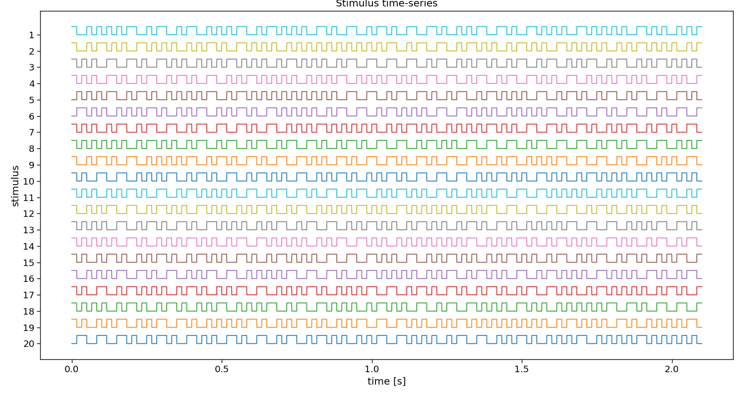
The cell below simulates some synthetic c-VEP data in response to a circularly shifted m-sequence.

FS = 120
PR = 60
SHIFT = 2

v = pyntbci.stimulus.make_m_sequence()
SHIFTS = np.arange(0, v.shape[1], SHIFT)
V = pyntbci.stimulus.shift(v, SHIFT)
V = np.repeat(V, FS // PR, axis=1)
N_CLASSES = V.shape[0]
CYCLE_SIZE = V.shape[1] / FS
LAGS = SHIFTS / PR

N_TRIALS = 1 * N_CLASSES
N_CHANNELS = 16
N_SAMPLES = int(2 * CYCLE_SIZE * FS)
N_COMPONENTS = 3
N_FILTER_BANDS = 4
ENCODING_LENGTH = 0.3
SEED = 42

X, y, V = pyntbci.eeg.generate_c_vep(
    N_TRIALS, N_CHANNELS, N_SAMPLES, FS, n_classes=N_CLASSES, stimulus=V, primary_channels=8, random_state=SEED
)

Inspect data

# Print data shapes
print("X", X.shape, "(trials x channels x samples)", X.dtype)  # EEG
print("y", y.shape, "(trials)", y.dtype)  # labels
print("V", V.shape, "(classes, samples)", V.dtype)  # codes
print("fs", FS, "Hz")  # sampling frequency
print("fr", PR, "Hz")  # presentation rate

# Visualize EEG data
i_trial = 0  # the trial to visualize
plt.figure(figsize=(15, 5))
plt.plot(np.arange(0, N_SAMPLES) / FS, np.arange(N_CHANNELS) + X[i_trial, :, :].T)
plt.xlim([0, 1])  # limit to 1 second EEG data
plt.xlabel("time [s]")
plt.ylabel("channel")
plt.title(f"Single-trial multi-channel EEG time-series (trial {i_trial})")
plt.tight_layout()

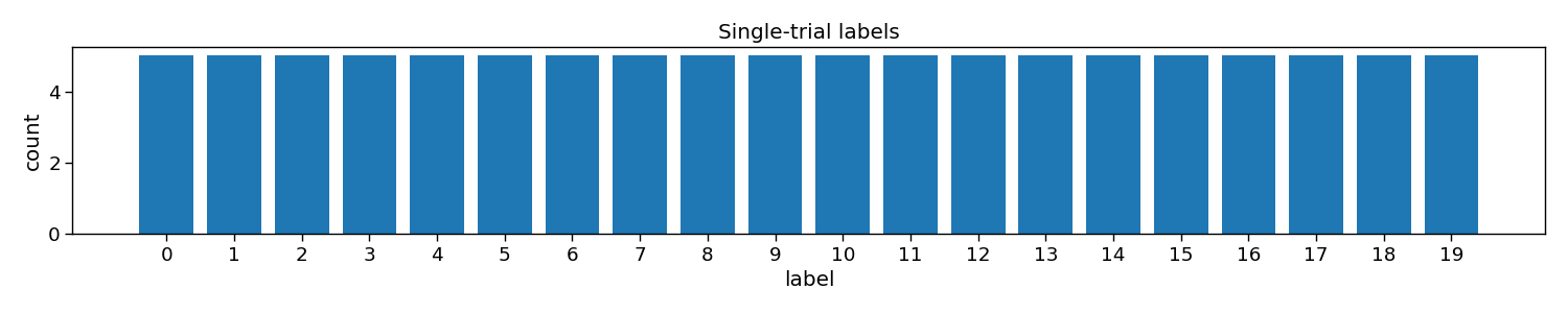
# Visualize labels
plt.figure(figsize=(15, 3))
hist = np.histogram(y, bins=np.arange(N_CLASSES + 1))[0]
plt.bar(np.arange(N_CLASSES), hist)
plt.xticks(np.arange(N_CLASSES))
plt.xlabel("label")
plt.ylabel("count")
plt.title("Single-trial labels")
plt.tight_layout()

# Visualize stimuli
fig, ax = plt.subplots(1, 1, figsize=(15, 8))
pyntbci.plotting.stimplot(V, fs=FS, ax=ax, plotfs=False)
fig.tight_layout()
ax.set_title("Stimulus time-series")

• 
• 
• 

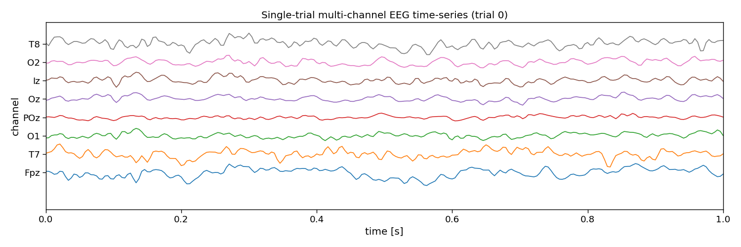
X (32, 16, 252) (trials x channels x samples) float32
y (32,) (trials) int64
V (32, 126) (classes, samples) uint8
fs 120 Hz
fr 60 Hz

Text(0.5, 1.0, 'Stimulus time-series')

ERP CCA

The full ERP CCA (eCCA) pipeline is implemented as a scikit-learn compatible class in PyntBCI in pyntbci.classifiers.eCCA. All it needs are the lags if a circular shifted code is used (not used here) in lags, the sampling frequency fs, and the duration of one period of a code as cycle_size.

When calling eCCA.fit(X, y) with training data X and labels y, the template responses are learned as well as the spatial filters eCCA.w_.

# Perform CCA
ecca = pyntbci.classifiers.eCCA(lags=LAGS, fs=FS, cycle_size=CYCLE_SIZE)
ecca.fit(X, y)
print("w: shape:", ecca.w_.shape, ", type:", ecca.w_.dtype)

# Plot CCA filter
fig, ax = plt.subplots(figsize=(5, 3))
ax.plot(np.arange(N_CHANNELS), ecca.w_)
ax.set_title("spatial filter")
ax.set_xlabel("channel")
ax.set_ylabel("weight")
ax.set_title("Spatial filter")

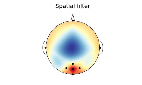
w: shape: (16, 1) , type: float32

Text(0.5, 1.0, 'Spatial filter')

Cross-validation

To perform decoding, one can call eCCA.fit(X_trn, y_trn) on training data X_trn and labels y_trn and eCCA.predict(X_tst) on testing data X_tst. In this section, a chronological cross-validation is set up to evaluate the performance of eCCA.

# Chronological cross-validation
n_folds = 4
folds = np.repeat(np.arange(n_folds), int(N_TRIALS / n_folds))

# Loop folds
accuracy = np.zeros(n_folds)
for i_fold in range(n_folds):
    # Split data to train and valid set
    X_trn, y_trn = X[folds != i_fold, :, :], y[folds != i_fold]
    X_tst, y_tst = X[folds == i_fold, :, :], y[folds == i_fold]

    # Train template-matching classifier
    ecca = pyntbci.classifiers.eCCA(lags=LAGS, fs=FS, cycle_size=CYCLE_SIZE)
    ecca.fit(X_trn, y_trn)

    # Apply template-matching classifier
    yh_tst = ecca.predict(X_tst)

    # Compute accuracy
    accuracy[i_fold] = np.mean(yh_tst == y_tst)

# Compute theoretical ITR (i.e., without inter-trial interval)
itr = pyntbci.utilities.itr(N_CLASSES, accuracy, N_SAMPLES / FS)

# Plot accuracy (over folds)
plt.figure(figsize=(15, 3))
plt.bar(np.arange(n_folds), accuracy)
plt.axhline(accuracy.mean(), linestyle="--", alpha=0.5, label="average")
plt.axhline(1 / N_CLASSES, color="k", linestyle="--", alpha=0.5, label="chance")
plt.xlabel("(test) fold")
plt.ylabel("accuracy")
plt.legend()
plt.title("Chronological cross-validation")
plt.tight_layout()

# Print accuracy (average and standard deviation over folds)
print(f"Accuracy: avg={accuracy.mean():.2f} with std={accuracy.std():.2f}")
print(f"ITR: avg={itr.mean():.1f} with std={itr.std():.2f}")

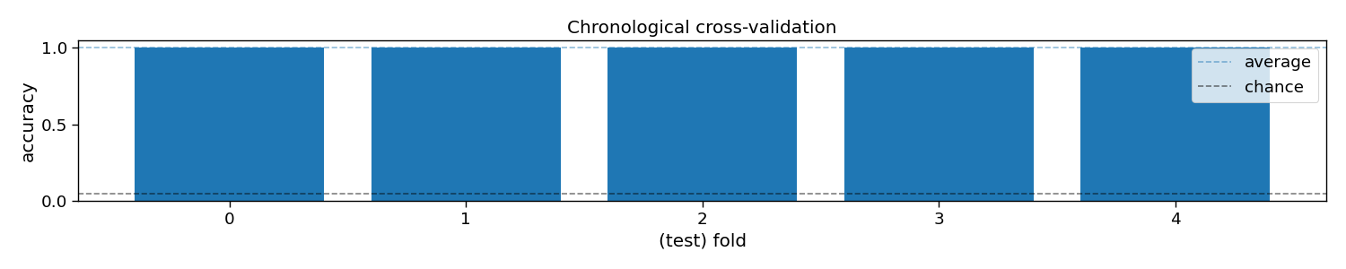
Accuracy: avg=1.00 with std=0.00
ITR: avg=142.9 with std=0.00

Learning curve

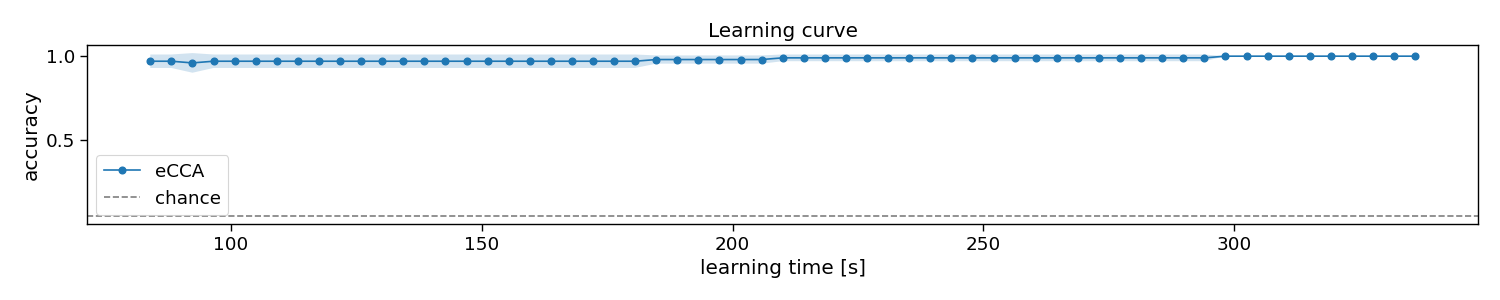
In this section, we will apply the decoder to varying number of training trials, to estimate a so-called learning curve. With this information, one could decide how much training data is required, or compare algorithms on how much training data they require to estimate their parameters.

# Chronological cross-validation
n_folds = 4
folds = np.repeat(np.arange(n_folds), int(N_TRIALS / n_folds))

# Set learning curve axis
train_trials = np.arange(1, 1 + np.sum(folds != 0))
n_train_trials = train_trials.size

# Loop folds
accuracy = np.zeros((n_folds, n_train_trials))
for i_fold in range(n_folds):
    # Split data to train and test set
    X_trn, y_trn = X[folds != i_fold, :, :], y[folds != i_fold]
    X_tst, y_tst = X[folds == i_fold, :, :], y[folds == i_fold]

    # Loop train trials
    for i_trial in range(n_train_trials):
        # Train classifier
        ecca = pyntbci.classifiers.eCCA(lags=LAGS, fs=FS, cycle_size=CYCLE_SIZE)
        ecca.fit(X_trn[: train_trials[i_trial], :, :], y_trn[: train_trials[i_trial]])

        # Apply classifier
        yh_tst = ecca.predict(X_tst)

        # Compute accuracy
        accuracy[i_fold, i_trial] = np.mean(yh_tst == y_tst)

# Plot results
plt.figure(figsize=(15, 3))
avg = accuracy.mean(axis=0)
std = accuracy.std(axis=0)
plt.plot(train_trials * N_SAMPLES / FS, avg, linestyle="-", marker="o", label="eCCA")
plt.fill_between(train_trials * N_SAMPLES / FS, avg + std, avg - std, alpha=0.2, label="_eCCA")
plt.axhline(1 / N_CLASSES, color="k", linestyle="--", alpha=0.5, label="chance")
plt.xlabel("learning time [s]")
plt.ylabel("accuracy")
plt.legend()
plt.title("Learning curve")
plt.tight_layout()

Decoding curve

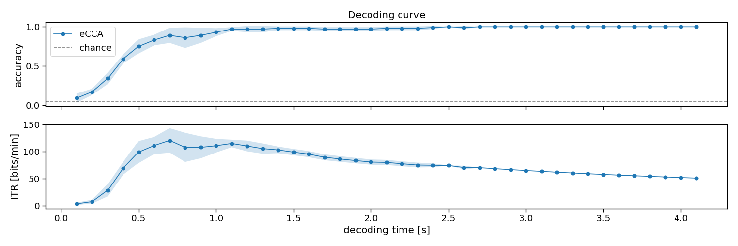
In this section, we will apply the decoder to varying testing trial lengths, to estimate a so-called decoding curve. With this information, one could decide how much testing data is required, or compare algorithms on how much data they need during testing to classify single-trials.

# Chronological cross-validation
n_folds = 4
folds = np.repeat(np.arange(n_folds), int(N_TRIALS / n_folds))

# Set decoding curve axis
segmenttime = 0.1  # step size of the decoding curve in seconds
segments = np.arange(segmenttime, N_SAMPLES / FS, segmenttime)
n_segments = segments.size

# Loop folds
accuracy = np.zeros((n_folds, n_segments))
for i_fold in range(n_folds):
    # Split data to train and test set
    X_trn, y_trn = X[folds != i_fold, :, :], y[folds != i_fold]
    X_tst, y_tst = X[folds == i_fold, :, :], y[folds == i_fold]

    # Setup classifier
    ecca = pyntbci.classifiers.eCCA(lags=LAGS, fs=FS, cycle_size=CYCLE_SIZE)

    # Train classifier
    ecca.fit(X_trn, y_trn)

    # Loop segments
    for i_segment in range(n_segments):
        # Apply classifier
        yh_tst = ecca.predict(X_tst[:, :, : int(FS * segments[i_segment])])

        # Compute accuracy
        accuracy[i_fold, i_segment] = np.mean(yh_tst == y_tst)

# Compute ITR
itr = pyntbci.utilities.itr(N_CLASSES, accuracy, np.tile(segments[np.newaxis, :], (n_folds, 1)))

# Plot results
fig, ax = plt.subplots(2, 1, figsize=(15, 5), sharex=True)
avg = accuracy.mean(axis=0)
std = accuracy.std(axis=0)
ax[0].plot(segments, avg, linestyle="-", marker="o", label="eCCA")
ax[0].fill_between(segments, avg + std, avg - std, alpha=0.2, label="_eCCA")
ax[0].axhline(1 / N_CLASSES, color="k", linestyle="--", alpha=0.5, label="chance")
avg = itr.mean(axis=0)
std = itr.std(axis=0)
ax[1].plot(segments, avg, linestyle="-", marker="o", label="eCCA")
ax[1].fill_between(segments, avg + std, avg - std, alpha=0.2, label="_eCCA")
ax[1].set_xlabel("decoding time [s]")
ax[0].set_ylabel("accuracy")
ax[1].set_ylabel("ITR [bits/min]")
ax[0].legend()
ax[0].set_title("Decoding curve")
fig.tight_layout()