Getting started

This getting started tutorial shows an example of how to use the PyntBCI library for analysing code-modulated responses [1]. This tutorial makes use of a small synthetic EEG dataset of EEG data. In this notebook, the reconvolution CCA (rCCA) method for decoding EEG is demonstrated, see [1] and [2].

References

[1] (1,2)

Martínez-Cagigal, V., Thielen, J., Santamaria-Vazquez, E., Pérez-Velasco, S., Desain, P., & Hornero, R. (2021). Brain–computer interfaces based on code-modulated visual evoked potentials (c-VEP): A literature review. Journal of Neural Engineering, 18(6), 061002. DOI: https://doi.org/10.1088/1741-2552/ac38cf

[2]

Thielen, J., Marsman, P., Farquhar, J., & Desain, P. (2021). From full calibration to zero training for a code-modulated visual evoked potentials for brain–computer interface. Journal of Neural Engineering, 18(5), 056007. DOI: https://doi.org/10.1088/1741-2552/abecef

[3]

Thielen, J., van den Broek, P., Farquhar, J., & Desain, P. (2015). Broad-Band visually evoked potentials: re(con)volution in brain-computer interfacing. PLOS ONE, 10(7), e0133797. DOI: https://doi.org/10.1371/journal.pone.0133797

import matplotlib.pyplot as plt
import numpy as np

import pyntbci

Simulate data

The cell below simulates some synthetic c-VEP data in response to a circularly shifted m-sequence. The dataset consists of: (1) The EEG data X that is a matrix of k trials, c channels, and m samples; (2) The labels y that is a vector of k trials; (3) The pseudo-random noise-codes V that is a matrix of stimuli with n classes and m samples. Note, the stimuli are upsampled to the EEG sampling frequency and contain only one stimulus-cycle. During a trial, however, the stimuli were repeated 2 times (2 stimulus cycles).

FS = 120
PR = 60
SHIFT = 2

v = pyntbci.stimulus.make_m_sequence()
SHIFTS = np.arange(0, v.shape[1], SHIFT)
V = pyntbci.stimulus.shift(v, SHIFT)
V = np.repeat(V, FS // PR, axis=1)
N_CLASSES = V.shape[0]
CYCLE_SIZE = V.shape[1] / FS
LAGS = SHIFTS / PR

N_TRIALS = 1 * N_CLASSES
N_CHANNELS = 16
N_SAMPLES = int(2 * CYCLE_SIZE * FS)
N_COMPONENTS = 3
N_FILTER_BANDS = 4
ENCODING_LENGTH = 0.3
SEED = 42

y = np.random.permutation(np.arange(N_TRIALS) % N_CLASSES)
X, y, V = pyntbci.eeg.generate_c_vep(
    N_TRIALS, N_CHANNELS, N_SAMPLES, FS, y=y, stimulus=V, primary_channels=8, random_state=SEED
)

Inspect data

# Print data shapes
print("X", X.shape, "(trials x channels x samples)", X.dtype)  # EEG
print("y", y.shape, "(trials)", y.dtype)  # labels
print("V", V.shape, "(classes, samples)", V.dtype)  # codes
print("fs", FS, "Hz")  # sampling frequency
print("fr", PR, "Hz")  # presentation rate

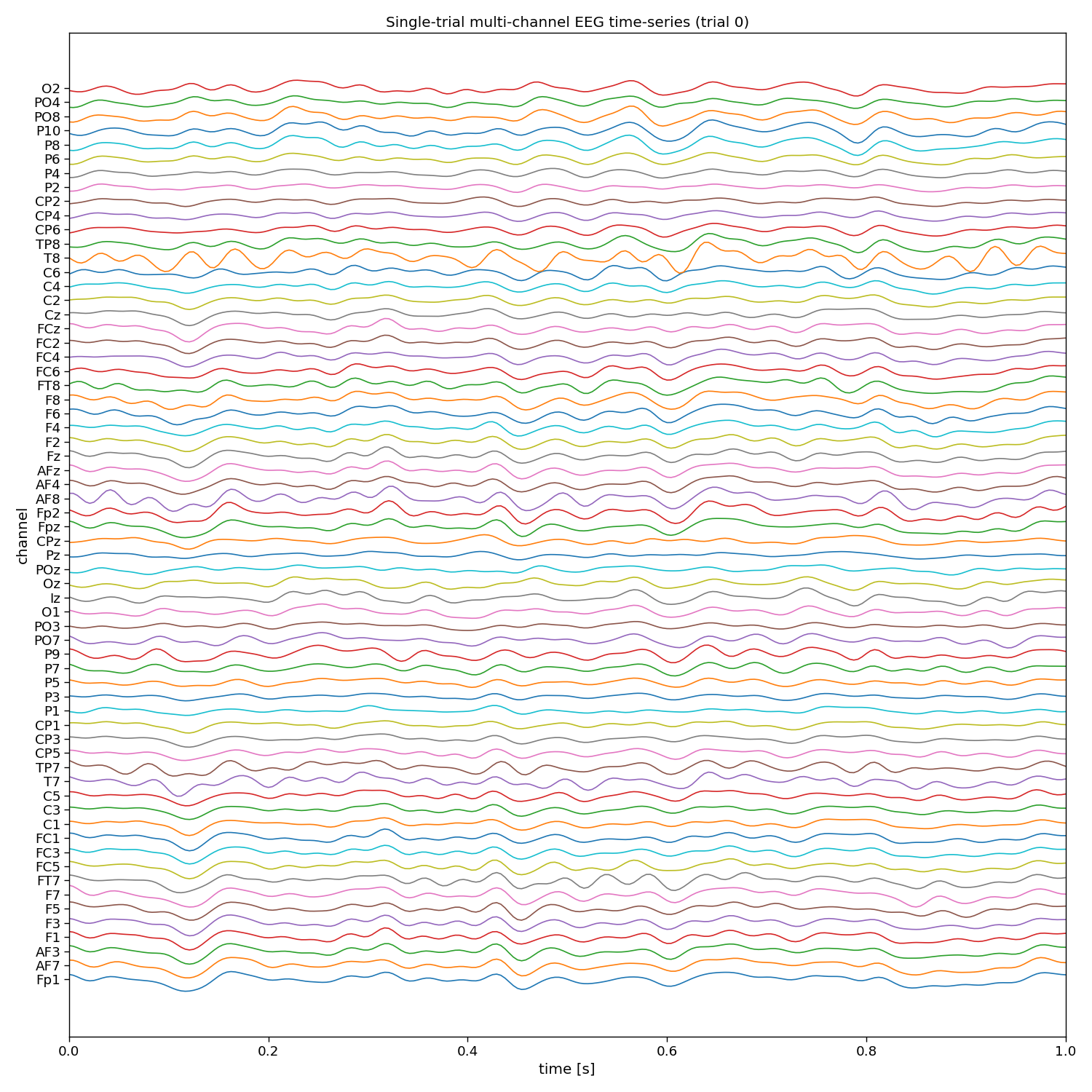
# Visualize EEG data
i_trial = 0  # the trial to visualize
plt.figure(figsize=(15, 5))
plt.plot(np.arange(0, N_SAMPLES) / FS, np.arange(N_CHANNELS) + X[i_trial, :, :].T)
plt.xlim([0, 1])  # limit to 1 second EEG data
plt.xlabel("time [s]")
plt.ylabel("channel")
plt.title(f"Single-trial multi-channel EEG time-series (trial {i_trial})")
plt.tight_layout()

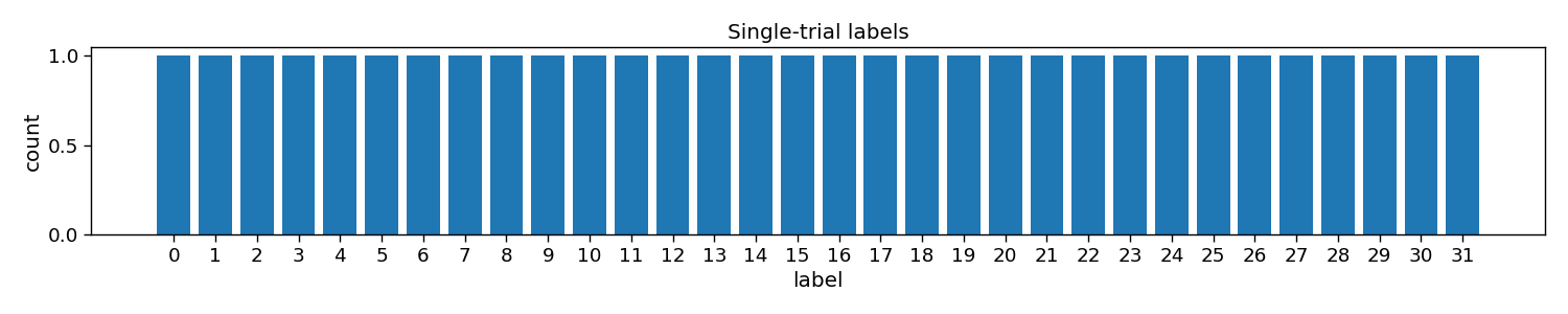
# Visualize labels
plt.figure(figsize=(15, 3))
hist = np.histogram(y, bins=np.arange(N_CLASSES + 1))[0]
plt.bar(np.arange(N_CLASSES), hist)
plt.xticks(np.arange(N_CLASSES))
plt.xlabel("label")
plt.ylabel("count")
plt.title("Single-trial labels")
plt.tight_layout()

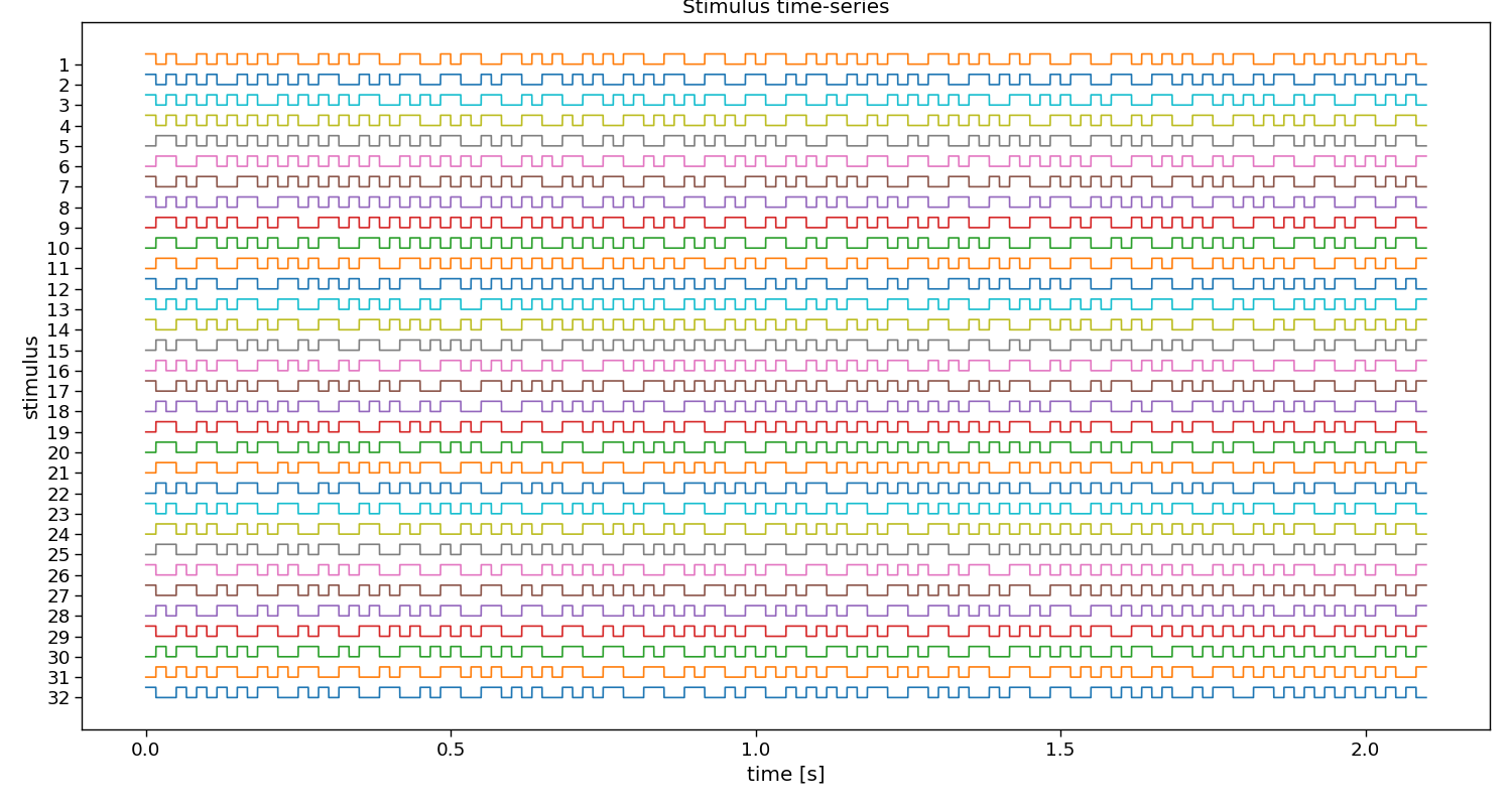
# Visualize stimuli
fig, ax = plt.subplots(1, 1, figsize=(15, 8))
pyntbci.plotting.stimplot(V, fs=FS, ax=ax, plotfs=False)
fig.tight_layout()
ax.set_title("Stimulus time-series")

• 
• 
• 

X (32, 16, 252) (trials x channels x samples) float32
y (32,) (trials) int64
V (32, 126) (classes, samples) uint8
fs 120 Hz
fr 60 Hz

Text(0.5, 1.0, 'Stimulus time-series')

The event matrix

The first step for reconvolution is to find within the sequences the repetitive events. This can be imposed “manually” by choosing the event definition that we believe the brain responds to. Here, the so-called “duration” event is used, which marks the length of a flash as the important piece of information. As the sequences in this dataset were modulated, there are only two events: a short and a long flash. Additionally, a third event is added that will account for the onset of a trial, during which all of a sudden the screen started flashing. The event matrix is a matrix of n classes, e events, and m samples.

Please, note that more event definitions exist, which can be explored with the event variable of rCCA. For instance, event=”contrast” is a useful event definition as well, which looks at rising and falling edges, generalising over the length of a flash.

# Create event matrix
E, events = pyntbci.utilities.event_matrix(V, event="duration")
print("E:", E.shape, "(classes x events x samples)")
print("Events:", ", ".join([str(event) for event in events]))

# Visualize event time-series
i_class = 0  # the class to visualize
fig, ax = plt.subplots(1, 1, figsize=(15, 3))
pyntbci.plotting.eventplot(V[i_class, :: int(FS / PR)], E[i_class, :, :: int(FS / PR)], fs=PR, ax=ax, events=events)
ax.set_title(f"Event time-series (code {i_class})")
plt.tight_layout()

# Visualize event matrix
i_class = 0
plt.figure(figsize=(15, 3))
plt.imshow(E[i_class, :, :], cmap="gray")
plt.gca().set_aspect(10)
plt.xticks(np.arange(0, E.shape[2], 60), np.arange(0, E.shape[2], 60) / FS)
plt.yticks(np.arange(E.shape[1]), events)
plt.xlabel("time [s]")
plt.title(f"Event matrix (class {i_class})")
plt.tight_layout()

• 
• 

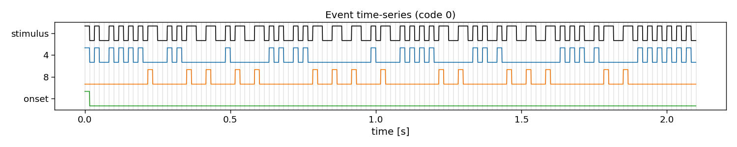
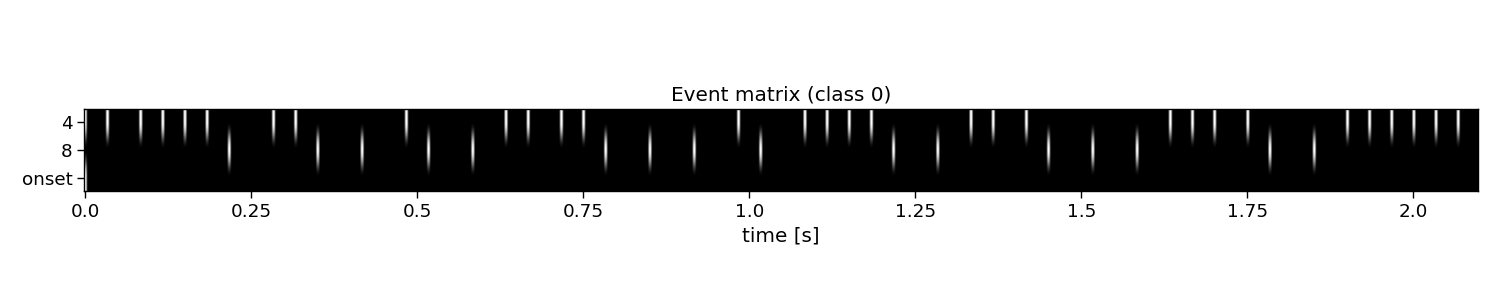
E: (32, 5, 126) (classes x events x samples)
Events: 2, 4, 6, 8, 12

The structure matrix

The second step for reconvolution is to model the expected responses associated to each of the events and their overlap. This is done in the so-called structure matrix (or design matrix). The structure matrix is essentially a Toeplitz version of the event matrix. It allows to model the c-VEP as the dot product of r (the transient response to an event) and M (the structure matrix for a specific class) for the ith class. The structure matrix is a matrix of n classes, l response samples, and m samples.

An important parameter here is the encoding_length argument. An easy abstraction is to assume the same length for the responses to each of the events. However, one could also set different lengths for each of the events.

# Create structure matrix
encoding_length = int(0.3 * FS)  # 300 ms responses
M = pyntbci.utilities.encoding_matrix(E, encoding_length)
print("M:", M.shape, "(classes x encoding_length*events x samples)")

# Plot structure matrix
i_class = 0  # the class to visualize
plt.figure(figsize=(15, 6))
plt.imshow(M[i_class, :, :], cmap="gray")
plt.xticks(np.arange(0, M.shape[2], 60), np.arange(0, M.shape[2], 60) / FS)
plt.yticks(np.arange(0, E.shape[1] * encoding_length, 12), np.tile(np.arange(0, encoding_length, 12) / FS, E.shape[1]))
plt.xlabel("time [s]")
plt.ylabel(events[::-1])
plt.title(f"Structure matrix (class {i_class})")
plt.tight_layout()

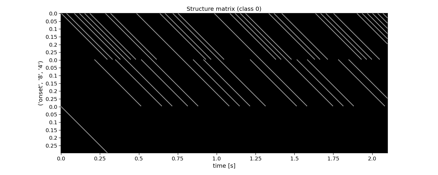
M: (32, 180, 126) (classes x encoding_length*events x samples)

Reconvolution CCA

The full reconvolution CCA (rCCA) pipeline is implemented as a scikit-learn compatible class in PyntBCI in pyntbci.classifiers.rCCA. All it needs are the binary sequences stimulus, the sampling frequency fs, the event definition event, the transient response size encoding_length and whether to include an event for the onset of a trial onset_event.

When calling rCCA.fit(X, y) with training data X and labels y, the full decomposition is performed to obtain spatial filters rCCA.w_ and temporal filter rCCA.r_.

Please note that the transient responses are concatenated in this temporal filter rCCA.r_. One can use rCCA.events_ to disentangle these and find which response is associated to which event.

# Perform CCA decomposition with duration event
encoding_length = 0.3  # 300 ms responses
rcca = pyntbci.classifiers.rCCA(stimulus=V, fs=FS, event="duration", encoding_length=encoding_length)
rcca.fit(X, y)
print("w: ", rcca.w_.shape, "(channels)")
print("r: ", rcca.r_.shape, "(encoding_length*events)")

# Plot CCA filters
fig, ax = plt.subplots(1, 2, figsize=(15, 3))
ax[0].plot(np.arange(N_CHANNELS), rcca.w_)
ax[0].set_title("spatial filter")
ax[0].set_xlabel("channel")
ax[0].set_ylabel("weight")
tmp = np.reshape(rcca.r_, (len(rcca.events_), -1))
for i in range(len(rcca.events_)):
    ax[1].plot(np.arange(int(encoding_length * FS)) / FS, tmp[i, :])
ax[1].legend(rcca.events_)
ax[1].set_xlabel("time [s]")
ax[1].set_ylabel("amplitude [a.u.]")
ax[1].set_title("Transient responses")
fig.tight_layout()

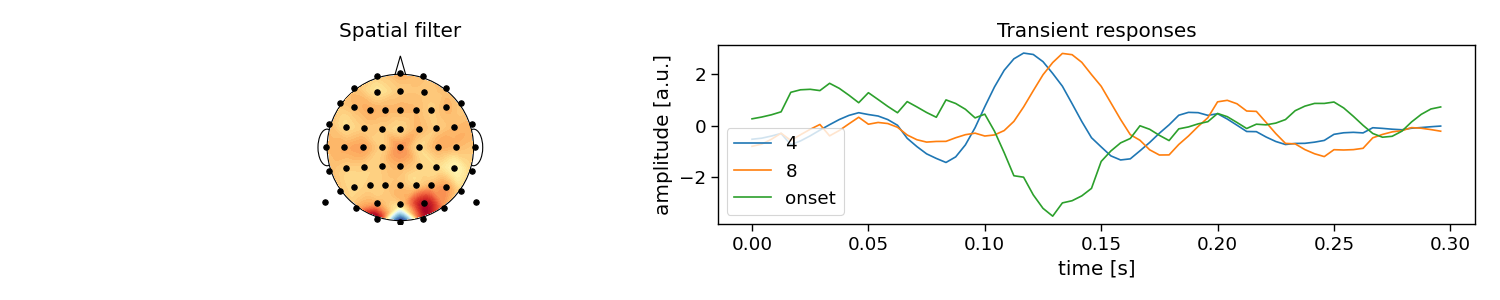
w:  (16, 1) (channels)
r:  (180, 1) (encoding_length*events)

Cross-validation

To perform decoding, one can call rCCA.fit(X_trn, y_trn) on training data X_trn and labels y_trn and rCCA.predict(X_tst) on testing data X_tst. In this section, a chronological cross-validation is set up to evaluate the performance of rCCA.

# Chronological cross-validation
n_folds = 4
folds = np.repeat(np.arange(n_folds), int(N_TRIALS / n_folds))

# Loop folds
accuracy = np.zeros(n_folds)
for i_fold in range(n_folds):
    # Split data to train and test set
    X_trn, y_trn = X[folds != i_fold, :, :], y[folds != i_fold]
    X_tst, y_tst = X[folds == i_fold, :, :], y[folds == i_fold]

    # Train template-matching classifier
    rcca = pyntbci.classifiers.rCCA(stimulus=V, fs=FS, event="duration", encoding_length=0.3)
    rcca.fit(X_trn, y_trn)

    # Apply template-matching classifier
    yh_tst = rcca.predict(X_tst)

    # Compute accuracy
    accuracy[i_fold] = np.mean(yh_tst == y_tst)

# Compute theoretical ITR (i.e., without inter-trial interval)
itr = pyntbci.utilities.itr(N_CLASSES, accuracy, N_SAMPLES / FS)

# Plot accuracy (over folds)
plt.figure(figsize=(15, 3))
plt.bar(np.arange(n_folds), accuracy)
plt.axhline(accuracy.mean(), linestyle="--", alpha=0.5, label="average")
plt.axhline(1 / N_CLASSES, color="k", linestyle="--", alpha=0.5, label="chance")
plt.xlabel("(test) fold")
plt.ylabel("accuracy")
plt.legend()
plt.title("Chronological cross-validation")
plt.tight_layout()

# Print accuracy (average and standard deviation over folds)
print(f"Accuracy: avg={accuracy.mean():.2f} with std={accuracy.std():.2f}")
print(f"ITR: avg={itr.mean():.1f} with std={itr.std():.2f}")

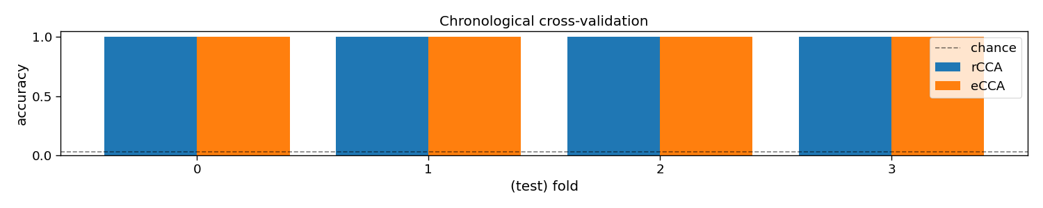
Accuracy: avg=1.00 with std=0.00
ITR: avg=142.9 with std=0.00